Two retrieval reports compare exactly the same ranked documents. One says list X is better; the other says list Y is better. Before looking for a changed model, check what the reports mean by a good result. A graded ranking metric needs a rule that turns relevance labels into numerical credit, as well as a rule for discounting lower positions.

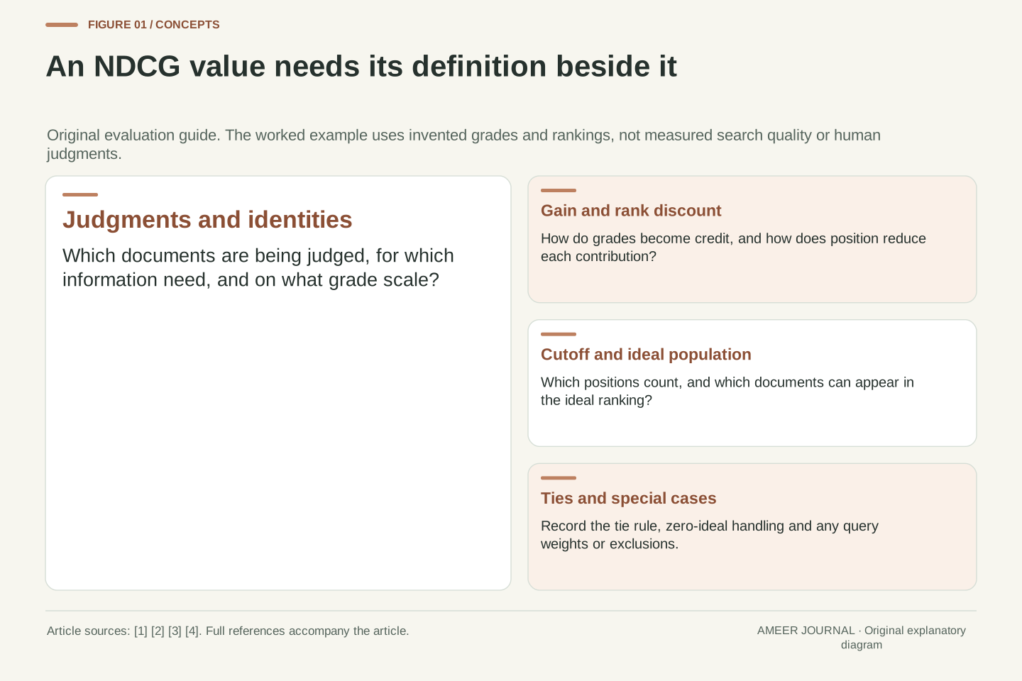
Normalized discounted cumulative gain, usually shortened to NDCG, combines those choices with a comparison against an ideal ranking. The scikit-learn documentation describes summing relevance scores in predicted order and dividing by the best possible discounted score. TensorFlow Ranking exposes separate gain and rank-discount functions [1][2]. The name alone does not supply every setting.

Our original example uses four imaginary documents and two fixed orders. With one gain rule, X wins. With another, Y wins. No search system, model or human assessment was run: all labels and rankings are stipulated. The calculation explains what must accompany a retrieval score before it can support a comparison.

NDCG is a normalized graded-ranking measure, but its interpretation requires a declared gain mapping, position discount, cutoff, judged universe and tie policy. Fixing the ranked outputs does not fix all those inputs. Changing the gain mapping can reverse an ordering between two lists without changing either list or its relevance labels.

Scikit-learn documents true-score accumulation under the predicted order and ideal normalization [1]. TensorFlow Ranking expresses DCG using explicit gain and rank-discount functions, with NDCG as a ratio to ideal DCG [2]. These documented interfaces motivate checking the full metric definition rather than treating the acronym as a complete contract.

The construction below uses one fully judged four-document universe, two stipulated permutations and two explicitly chosen gain functions. An original pure-Python calculation enumerates all twenty-four permutations to check the ideal values. It does not execute either library, collect real relevance judgments or evaluate a retriever. Its result is a precise example of metric-definition sensitivity.

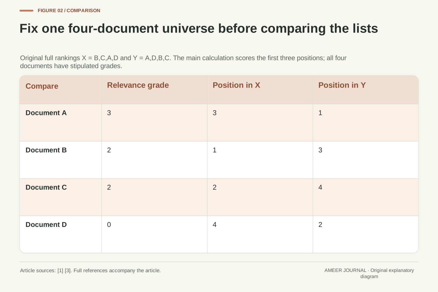
Give document A relevance grade three, B grade two, C grade two and D grade zero. Think of zero as irrelevant to the stated need, two as useful and three as very useful. These descriptions explain our invented scale; they are not observations about real documents. Grade one is allowed by the scale but does not occur in this four-document collection.

List X orders the documents B, C, A, D. List Y orders them A, D, B, C. Both complete lists contain the same four identities exactly once. At a cutoff of three, X shows B, C and A, while Y shows A, D and B. The cutoff matters because C falls outside Y's scored portion.

Elastic's ranking-evaluation guide associates document ratings with each particular query and the user's information need [3]. A grade therefore belongs to a defined judgment task. Our fixed labels let us compare the arithmetic while avoiding any claim that an assessor actually preferred these documents or that this scale measures a user's satisfaction.

Define universe U={A,B,C,D} with relevance vector r(A)=3, r(B)=2, r(C)=2 and r(D)=0. Every identity is judged, no document is duplicated, and the evaluation concerns one fixed information need. Ranking X=(B,C,A,D) and ranking Y=(A,D,B,C) are full permutations. The principal comparison uses k=3.

The rating definition is distinct from the ranking score. Elastic documents query-specific ratings on a user-defined integer scale [3]. Here the integers are assigned teaching values. They are not predicted probabilities, evidence of an interval utility scale or the output of a human or automated labeling procedure.

Keeping U fixed makes the ideal denominator common to X and Y under each chosen gain function. Their top-three prefixes have different memberships, although their complete permutations share the same universe. This distinction will matter when interpreting a conditional candidate-set evaluation later. We do not silently redefine the judged population to match whichever results a particular list happens to return.

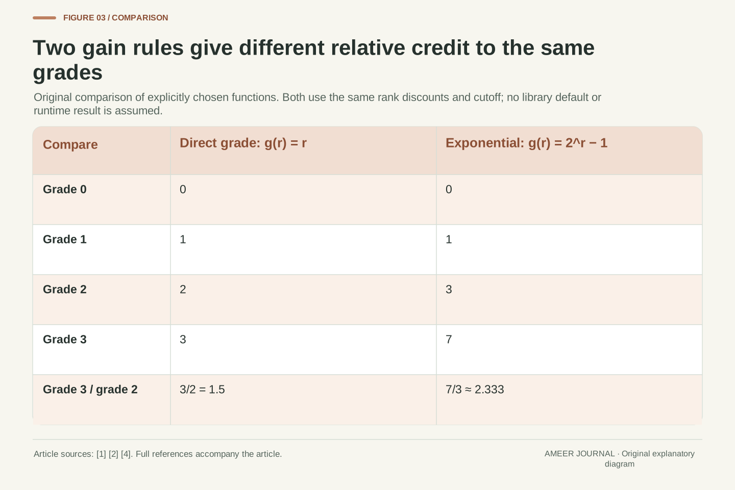
A gain rule says how much credit a relevance grade earns before position is considered. Our first rule uses the grade directly: zero earns zero, one earns one, two earns two and three earns three. A rank discount then gives less weight to the same gain when it appears farther down the list.

Use the discount “one divided by log base two of rank plus one.” At rank one its value is one; at rank two it is about 0.63093; at rank three it is one-half. Multiply each document's gain by its position's discount, then add the contributions. That total is our discounted cumulative gain, or DCG.

Finally, divide by the highest DCG possible for the same judged collection, gain rule and cutoff. This produces our NDCG when the ideal value is positive. The documented metric separates these roles [1][2]. Our displayed numbers follow the stated formula, rather than an assumption that any software setting with the same name must reproduce them.

For an ordered list π and one-based rank i, define d(i)=1/log₂(i+1) and DCG_g@k(π)=Σᵢ₌₁ᵏ g(r(πᵢ))d(i). If fewer results are supplied, the sum contains only those positions. The initial gain is g_L(r)=r. Discount values for ranks one through three are 1, a=1/log₂3≈0.630929754 and 1/2.

Define IDCG_g@k as the maximum DCG under all permutations of the declared U. For positive IDCG, NDCG_g@k=DCG_g@k/IDCG_g@k. This is the explicit specialization used in the original calculations; TensorFlow documents the more general gain-times-discount decomposition, while scikit-learn describes ideal normalization [1][2].

With our nonnegative gains and decreasing discounts, sorting by descending gain achieves the maximum. To see why, give positions after the cutoff discount zero. For two ranks i<j holding gains u<v, swapping them increases DCG by (v−u)(d(i)−d(j)), which is nonnegative. Repeating such swaps produces descending gain order; equal gains need no preferred order. A and then B/C in either order provide the ideal top three. Enumeration over all twenty-four orders checks this result. The denominator uses the same k and gain function as the numerator; mixing their definitions would describe a different ratio.

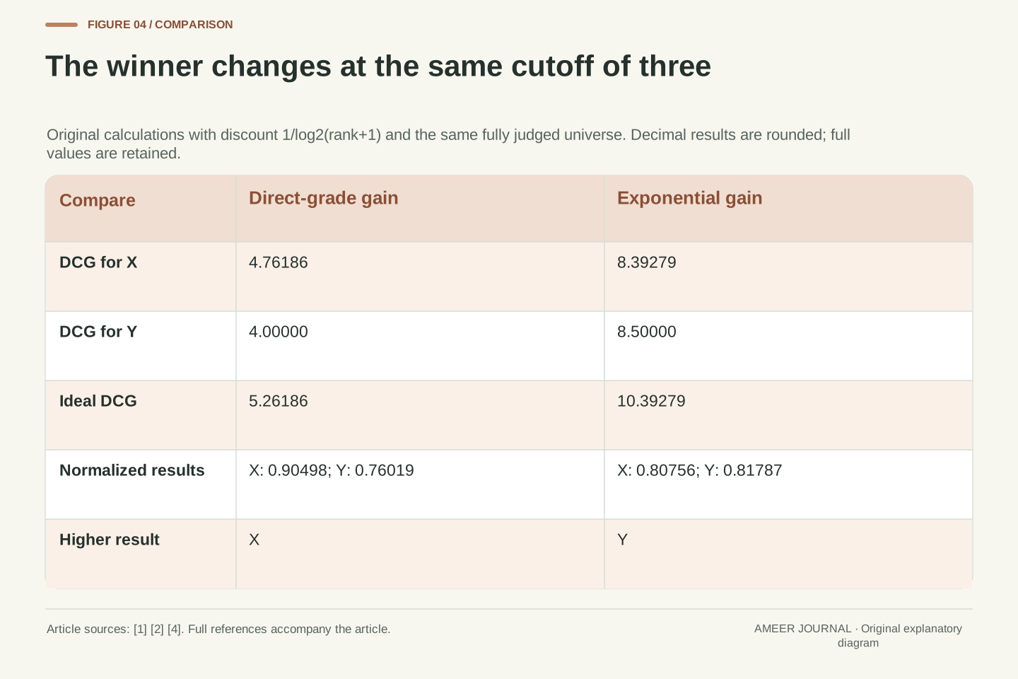
For list X, the first three grades are two, two and three. Their discounted contributions are 2, about 1.26186 and 1.5. Add them to get a DCG of approximately 4.76186. List Y begins with grades three, zero and two, giving contributions 3, 0 and 1. Its DCG is exactly 4.

The ideal top three place A first, then B and C. Their grades are three, two and two, so ideal DCG is 3 plus about 1.26186 plus 1, or 5.26186. Dividing both list totals by this same ideal gives X approximately 0.90498 and Y approximately 0.76019. Under this declared rule, X ranks higher.

The result gives credit to X's two useful early documents as well as its very useful document in third place. Y places the highest-grade document first but spends second place on a zero-grade item. This explanation follows from our chosen gain and discount values. It is not a measured preference or a universal reason to favor one result pattern.

At k=3, X has DCG_L=2+2a+3/2=3.5+2a≈4.761859507. Y has DCG_L=3+0a+2/2=4. The ideal is IDCG_L=3+2a+2/2=4+2a≈5.261859507. Thus NDCG_L(X)≈0.904976558 and NDCG_L(Y)≈0.760187533.

Because the denominator is shared and positive, the normalized ordering matches the DCG ordering. X's DCG advantage is −1/2+2a≈0.761859507. The calculation values two grade-two documents near the top strongly enough to compensate for moving the grade-three document from rank one to rank three, while Y's zero-grade second result contributes nothing.

No score is a probability that a generated answer is correct. These are ratios of discounted gains under supplied relevance values. They are also not proportions of relevant documents: under a separate positive-grade binary rule, X has three relevant top-three items and Y has two. That count discards the grade distinctions that this DCG computation retains.

Now keep every grade, document and position unchanged, but give each grade the gain “two raised to that grade, minus one.” Grades zero, one, two and three become gains zero, one, three and seven. TensorFlow documents this function as an option for defining NDCG gain [4]. We are choosing it explicitly, not claiming that every NDCG implementation uses it.

X's first three gains are now 3, 3 and 7. Its DCG becomes 3 plus about 1.89279 plus 3.5, or 8.39279. Y's gains are 7, 0 and 3, giving 7 plus 0 plus 1.5, or 8.5. The ideal gains are 7, 3 and 3, producing ideal DCG of about 10.39279.

After normalization, X scores approximately 0.80756 and Y approximately 0.81787. Y now leads. Nothing was retrieved again and no label was corrected. The change comes entirely from a rule that gives the highest grade substantially more credit relative to the next grade.

Choose g_E(r)=2ʳ−1, yielding gains (0,1,3,7) for grades (0,1,2,3). TensorFlow's documented pow_minus_1 function computes this transformation and can define gain_fn [4]. The example uses it as a declared convention; it does not infer a default from a constructor parameter or run the TensorFlow metric.

At k=3, DCG_E(X)=3+3a+7/2=6.5+3a≈8.392789261. DCG_E(Y)=7+0a+3/2=8.5. IDCG_E=7+3a+3/2=8.5+3a≈10.392789261. Therefore NDCG_E(X)≈0.807558881 and NDCG_E(Y)≈0.817874758.

The difference DCG_E(X)−DCG_E(Y)=−2+3a≈−0.107210739 is negative, whereas the corresponding linear-gain difference was positive. This is an exact ordering reversal with floating-point values shown only for readability. The full identity, grade, rank, contribution and denominator records remain available for independent recomputation under the same mathematical definitions.

It is tempting to expect normalization to make the two gain rules interchangeable. It does make each ideal ranking score one. But each rule defines its own ideal and its own tradeoff between grades. It does not make the credit for a grade-three item mean the same thing under both rules.

With direct grades, grade three earns one-and-a-half times the gain of grade two: three divided by two. With the second rule, it earns seven-thirds as much, about 2.333 times. Those relative values change how much a first-place A can compensate for other positions. Multiplying the old gains by one fixed number could not create this change in their ratio.

For each rule, X and Y share one positive ideal denominator. Dividing by that common value preserves whichever list already has the higher DCG. The normalization does not undo the changed preference built into the gains. If labels are only zero and one, however, both gain rules give the same values. A binary example would miss the difference exposed by our grades two and three. Include genuinely graded cases when checking a graded metric.

Ideal normalization anchors the maximum at one within a defined evaluation problem. It does not identify distinct utility mappings. The ratio g_L(3)/g_L(2)=3/2 differs from g_E(3)/g_E(2)=7/3, so g_E is not a positive scalar multiple of g_L on the observed grades.

For any fixed positive constant c, replacing g with cg scales both DCG and IDCG by c and leaves their ratio unchanged. The original calculation verifies this with c=7 for both mappings and all four cutoffs. By contrast, the nonlinear gain change modifies relative contributions, so the new numerator and denominator do not simply share one canceling factor.

Within each mapping, the common positive ideal preserves the sign of the X-minus-Y DCG difference. Consequently normalization cannot remove the demonstrated reversal. On binary labels r∈{0,1}, however, g_L(r)=g_E(r). A binary-only verification case cannot distinguish these gain implementations, while our grade-two and grade-three records can. These are properties of the declared ratios, not evidence that one convention is correct for every need. The interpretation of graded usefulness must justify the chosen convention.

The numbers used to order results are different from the relevance grades used to evaluate them. Imagine assigning ordering scores 40, 30, 20 and 10 to the documents in X's order. Replace each ordering score with ten times its old value plus seven. The numbers change, but their descending order remains B, C, A, D.

Our NDCG uses that order and the fixed relevance grades. It therefore stays the same. A larger uncalibrated ordering score is not automatically a larger gain in this evaluation. Scikit-learn's interface distinguishes the true relevance values from the predicted scores that induce the ordering [1]. Confusing those two inputs would change the question being measured.

There is another cancellation in our exact formula: changing the logarithm base consistently in both DCG and ideal DCG multiplies all discounts by one common factor. The normalized ratio is unchanged. Neither cancellation applies to changing which documents are returned, their positions, their grades or the relative gain assigned to different grades.

Assign predicted scores s_X(B)=40, s_X(C)=30, s_X(A)=20 and s_X(D)=10. The strictly increasing affine transform s′=10s+7 preserves the permutation. Because our DCG consumes relevance gains at ranks rather than predicted-score magnitudes, every resulting NDCG is unchanged. This accords with the documented separation between y_true and order-inducing y_score [1].

Similarly, replacing log₂(i+1) with log_b(i+1), for b>1, scales every discount by log₂b. Using that same base in the numerator and ideal cancels the factor. The original arithmetic checks bases e and ten for both gain mappings and cutoffs one through four.

These invariances have explicit assumptions: the score transform preserves all ordering and tie relationships, and the logarithm change is applied consistently to a positive-denominator ratio. A different discount shape, changed cutoff, new tie or nonlinear relevance-to-gain mapping is not covered by these arguments. Distinguish a harmless representation change from a change to the evaluation's preferences.

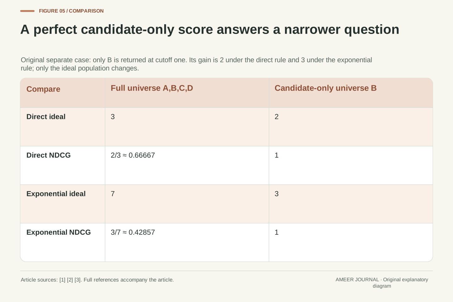
Suppose a retrieval stage returns only B. At cutoff one, B earns gain two under the direct-grade rule. Relative to our full judged collection, the ideal first document is A with gain three, so the score is two-thirds. Under the second gain rule, B earns three and A earns seven, giving three-sevenths.

Now redefine the evaluation population to contain only the returned B. B is necessarily the best item in that one-item set. Dividing by that smaller set's ideal produces one under either rule. The returned document has not improved. The denominator now answers a narrower question.

A candidate-only measure can be useful for examining ordering within an already chosen pool. It should not be presented as the same full-collection retrieval result. Our example has complete ratings for all four documents, making the missing A visible in the first denominator. Keep the evaluated population beside the score so a perfect conditional ranking is not mistaken for complete retrieval success.

For returned list (B) at k=1, full-universe IDCG_L is 3 and DCG_L is 2, giving 2/3. Exponential values are IDCG_E=7 and DCG_E=3, giving 3/7. These denominators use the declared U, including relevant identities absent from the returned list.

If the judged universe is redefined as U′={B}, both normalized scores become one because B is ideal within U′. This is a conditional evaluation of a different population. It is not algebraically inconsistent, but it is not interchangeable with the original full-universe question. The distinction can separate upstream candidate coverage from downstream ordering within a supplied pool.

The example assumes known grades for all four identities; it does not solve incomplete judging in a large corpus. A real report must state how its judged universe and ideal are constructed. Merely passing the returned items into a metric cannot establish that the resulting denominator represents every relevant item in the intended search population.

The symbol “at three” means that only the first three returned positions contribute. It does not mean that the ideal can use four positions or that every result shown elsewhere on a page was evaluated. The scikit-learn documentation explicitly describes a cutoff and an ideal normalization that takes that cutoff into account [1].

Extend our direct-grade calculation to cutoff four. X adds D, whose gain is zero, so its score remains about 0.90498. Y adds C at rank four. Its extra contribution is two divided by log base two of five, about 0.86135. Y's DCG becomes about 4.86135 and its NDCG about 0.92389. The ideal is unchanged because its fourth item is zero-grade D.

Y therefore overtakes X under the direct-grade rule at this larger cutoff. This is a separate change from the earlier gain-rule comparison, which held the cutoff fixed at three. Record one change at a time so a gain choice and a result-depth choice do not become indistinguishable explanations for a new score.

NDCG@k requires truncation of the observed and ideal accumulations at the same k. The scikit-learn API and examples explicitly retain that normalization boundary [1]. In the original universe, extending from k=3 to k=4 leaves the ideal DCG unchanged under either mapping because the added ideal item has zero gain.

For linear gain, DCG_L@4(X)=4.761859507 remains unchanged. Y adds 2/log₂5≈0.861353116, reaching DCG_L@4(Y)≈4.861353116. Dividing by the unchanged 5.261859507 ideal gives NDCG_L@4(Y)≈0.923885009, above X's 0.904976558.

This cutoff effect should remain separate from the fixed-k gain reversal. The original main comparison alters g while holding k=3; this extension alters k while holding g=g_L. Neither result is an empirical quality gain. Both demonstrate why a metric configuration and the complete result identities are needed to explain a changed report.

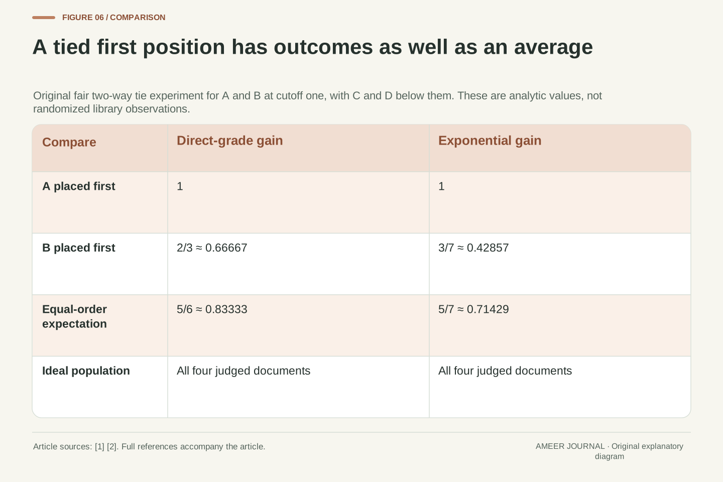
Create a separate ordering-score example in which A and B tie for first place, with C and D below them. Keep cutoff one. If A is selected first, the direct-grade normalized score is one. If B is selected first, it is two-thirds. The labels and tied scores alone do not choose between those displayed outcomes.

Under our explicitly chosen fair two-way tie experiment, average the two possible results. The expected direct-grade value is five-sixths, about 0.83333. With the exponential gain, the alternatives are one and three-sevenths, giving an expectation of five-sevenths, about 0.71429. These are calculated expectations, not observed randomized library runs.

Tie policy is a real interface distinction: scikit-learn documents averaging ties by default and warns about ignoring ties when they exist, while TensorFlow's metric description says score ties are broken randomly [1][2]. Preserve the actual policy used in a report. One realized order and an average across possible orders are different reported quantities.

Let A and B share the largest predicted score while C and D rank strictly below them. At k=1, the possible linear NDCGs are {1,2/3}; the possible exponential values are {1,3/7}. Our separate experiment assigns equal probability to the two top-order resolutions, yielding expectations 5/6 and 5/7 respectively.

This expectation is analytically enumerated over two equally weighted orderings. No random generator or library metric is executed, and uniformity is our declared assumption rather than an inferred implementation guarantee. The ideal remains the full-universe top-one value, so the only changing input is which tied document occupies the scored position.

The retained scikit-learn examples describe default tie averaging and the invalidity of assuming away existing ties; TensorFlow's definition describes random tie breaking [1][2]. These documented scopes support retaining the tie convention. They do not establish that one observed randomized result must equal its expectation or that all libraries share an identical treatment of tied cutoffs.

Imagine a new judgment task in which every document has grade zero. Both our gain rules then give DCG zero and ideal DCG zero. The raw ratio is zero divided by zero, which is undefined. A reporting system needs an explicit convention for this case, such as a documented value or an eligibility rule; this article does not assign one convention to every implementation.

That differs from returning no documents for our original positive-grade collection. Under our defined empty-sum rule, the numerator is zero but the ideal remains positive, so the normalized value is zero. An empty result and an all-zero judgment universe therefore reach different mathematical situations.

An unrated document is different again. It has no established grade in the record. Our four-document calculation avoids that issue by stipulating every label. In a real evaluation, record how missing judgments are handled rather than silently relabeling “unknown” as “irrelevant.” Also preserve the allowed grade range; negative values can break the usual normalized range described by the API [1].

If r(d)=0 for every d in U, both selected gain functions give DCG=IDCG=0. The ratio is undefined before a reporting convention is applied. The original record stores this as an unresolved mathematical ratio, not as an asserted scikit-learn, TensorFlow or Elastic return value.

For a different case with the original positive-grade U and no returned items, the empty numerator is zero while IDCG@k is positive, so the declared ratio is zero. These cases should not be conflated through a generic “nothing relevant returned” label. Their denominators contain different information.

Unjudged identities require another explicit policy; they are not negative or zero judgments by definition. The fixture's complete labels remove that uncertainty rather than estimating it. Likewise, the bounded-range reasoning assumes nonnegative gains and a valid positive ideal. Scikit-learn warns that negative true values can produce outputs outside the usual zero-to-one interval [1]. No conclusion here extends the four-document calculation to incomplete, negative-grade or differently weighted inputs without redefining the account.

A useful report names the information need, document identities, relevance grades, result order, gain rule, rank discount, cutoff, ideal population and tie treatment. If it combines several queries, it should also identify their weights and any excluded cases. Elastic's documentation keeps query-specific ratings and per-query results visible [3]; a single average cannot replace those underlying records.

Our main result is now reproducible. At cutoff three, direct grades give X about 0.90498 and Y about 0.76019. The exponential gain gives X about 0.80756 and Y about 0.81787. Both comparisons follow their declared definitions. The disagreement identifies a changed preference in the metric, not a changed retrieval run.

NDCG still evaluates ordering relative to the supplied judgments. It does not prove that a source is accurate, that a passage contains every necessary qualification, or that a generated answer uses the evidence correctly. Those questions need their own checks. Preserve the metric's useful, specific conclusion without stretching it into a complete assessment of a RAG application.

Retain the query or information-need identifier, judged universe, identity-to-grade mapping, complete predicted order, gain function, discount function, k, ideal construction, tie policy and zero-ideal handling. For an aggregate, retain query eligibility and weighting as well. The documented query-specific rating and detailed-result structure illustrates why the component records matter [3].

The original k=3 records establish NDCG_L(X)>NDCG_L(Y) but NDCG_E(X)<NDCG_E(Y), with no changes to U, grades or permutations. Separate extensions show candidate-conditional normalization, cutoff sensitivity, tie expectations and scaling invariances. Each conclusion is attached to an explicit change or fixed assumption rather than to an unexplained dashboard difference.

The calculation validates the metric account only. Supplied grades may still be unsuitable for a different need, and a high score does not validate the factual content of retrieved documents or a downstream answer. Keep those evaluation predicates separate. A reconstructible ranking measure can inform a defined retrieval decision without becoming a claim of general model quality or complete application correctness.