A model can have frozen weights and still produce different outputs on repeated passes. It can also change some of its stored state while those weights remain untouched. Neither observation automatically proves that the freeze setting failed. The setting may control a different part of the calculation from the one you are watching.

Fine-tuning adapts an existing model to a task. Hugging Face’s training guide describes that process and the need to evaluate the resulting task performance [5]. Here we examine a narrower question: when some weights are meant to stay fixed, which other controls still matter? We will separate weight updates, recorded derivatives, training behavior and stored running statistics.

The examples use two scalar weights, a two-number dropout input and a tiny batch-normalization calculation. They are original teaching examples, not measurements from a trained AI system. Their small size lets us follow every number. The main references are PyTorch 2.15 documentation and the Transformers 4.56.0 guide; this article does not claim that these are the newest installed versions.

Freezing is often used as shorthand for several different constraints: no parameter update, no parameter-gradient accumulation, no autograd recording, unchanged forward behavior or unchanged module state. Those constraints are not equivalent. A reproducible fine-tuning configuration must identify which of them it actually imposes.

Hugging Face describes fine-tuning as adaptation of a pretrained model and treats task evaluation as a separate part of the training workflow [5]. This article addresses the controls around that adaptation, using PyTorch 2.15 semantics for parameter flags, gradient modes and module modes. Transformers 4.56.0 supplies contextual training documentation rather than an executed training recipe.

Three original mathematical fixtures expose the distinctions: a scalar composition, an exhaustive two-element dropout enumeration and selected BatchNorm1d statistics. No framework, external model, dataset or benchmark was run. The fixtures stipulate fresh unset gradients and exclude unmentioned mutations. Their conclusions concern the stated calculations; they do not establish generalization quality, memory savings, speed or the correctness of an arbitrary training implementation.

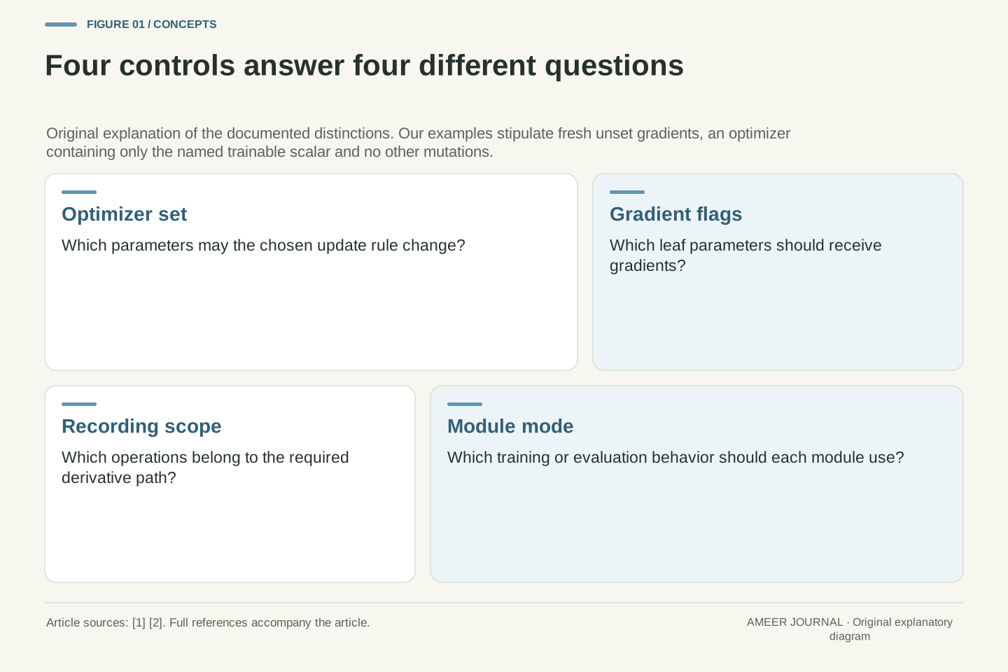
First ask which weights the update rule may change. In our examples, the optimizer receives only the weight named as trainable. Second ask which leaf weights should receive calculated gradients. PyTorch provides the requires_grad setting for that purpose [1, 2]. A gradient is a local instruction about how the loss changes when a value changes; it is not itself a weight update.

Third ask whether the operations needed for those gradients are being recorded. A no_grad region suppresses that recording [1]. Fourth ask how a module should behave on its forward pass. The train and eval settings affect modules with different training and evaluation behavior, including dropout and batch normalization [2].

These questions can have different answers in the same system. A weight may stay fixed while its operation remains necessary for a gradient flowing toward an earlier trainable weight. A module may use evaluation behavior while gradients are still being calculated. Writing the four choices separately makes a configuration much easier to understand than a single label saying frozen.

Distinguish the optimizer’s parameter set, leaf-gradient eligibility, operation recording and module behavior. The first defines which tensors the chosen update procedure is allowed to modify. The requires_grad flag controls gradient participation; in ordinary grad mode, requested leaf gradients accumulate in their .grad fields [1]. Neither a nonzero derivative nor its accumulation constitutes an optimizer step.

Recording is another control. Operations inside no_grad are excluded from the backward graph even when an input would otherwise require a gradient [1]. Module.train and Module.eval instead choose behavior implemented by particular modules. They are not substitutes for gradient-mode controls [1, 2].

For the teaching calculations, begin with no pre-existing gradients, place only the named trainable scalar in the optimizer and allow no other mutation. This makes the intended freeze unambiguous. The article does not claim that toggling a flag can neutralize arbitrary optimizer behavior, old gradient values or direct assignments. A useful configuration records these separate decisions instead of inferring all of them from one parameter flag.

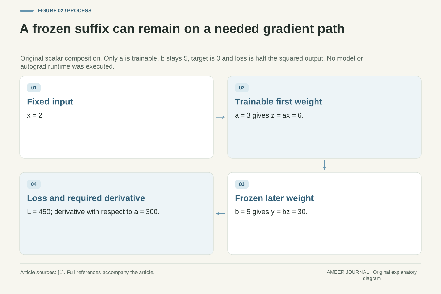
Consider a two-step calculation. Multiply input x by weight a, then multiply the result by weight b. Set x to 2, a to 3 and b to 5. The output is 30. Our target is zero, and the loss is half the squared output, giving 450.

Now freeze b and allow only a to change. The effect of changing a still passes through multiplication by 5. The loss gradient for a is 300. Taking one deliberately chosen step of 0.001 gives a new a of 2.7. With b still exactly 5, the output becomes 27 and the loss becomes 364.5. These are arithmetic results from the stated rule, not evidence that a real model has improved.

The important point is the path. PyTorch records an operation in ordinary grad mode when at least one input requires a gradient [1]. Even if b does not need its own gradient, the input arriving from a does. Freezing b therefore does not mean removing that multiplication from the derivative calculation needed for a.

Define y=bax and L=y²/2 with x=2, a=3 and b=5. Treat a as the only trainable leaf and b as a fixed leaf. Then y=30, L=450 and ∂L/∂a=b²ax²=300. The derivative depends on b’s value even though no gradient for updating b is requested.

An explicit gradient-descent step with learning rate 0.001 gives a′=3−0.001×300=2.7. Holding b fixed produces y′=27 and L′=364.5. The derivation is exact for this scalar quadratic. It is neither an autograd execution nor an empirical claim about adaptation or held-out performance.

The relevant PyTorch rule is input-specific: an operation is recorded in default grad mode if at least one input requires grad [1]. At the multiplication by b, the intermediate z=ax has a dependency on a. The backward path needs ∂y/∂z=b. No gradient accumulation into b is required for that chain rule. A frozen suffix can therefore remain part of the graph needed to optimize an earlier trainable component.

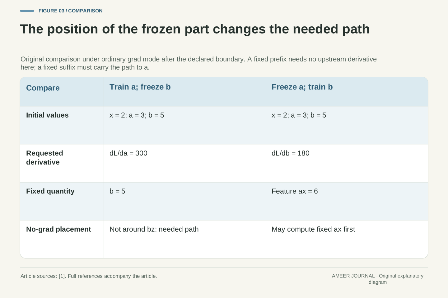
Suppose we keep the same arrangement but perform the final multiplication by b inside no_grad. That tells the framework not to record this operation. The loss no longer has the recorded route through that multiplication back to a. Leaving a marked trainable does not rebuild the missing route afterward [1].

Now change the learning problem. Freeze a at 3 and train only the later weight b. The input x is fixed, and we do not want gradients for x or a. The first step simply provides the fixed feature 3×2=6. We can calculate that feature without recording its history, then multiply it by trainable b in ordinary grad mode. The gradient for b is still available; in our initial example it is 180.

These two cases explain why advice to disable recording around every frozen layer is incomplete. A frozen prefix can be a fixed feature calculation when no learning signal needs to pass through it. A frozen suffix can still sit between the loss and an earlier trainable weight. Draw the required path before choosing the boundary.

Place only y=bz inside no_grad, where z=ax was computed from trainable a. That multiplication is not recorded. Consequently the resulting loss has no recorded path through it to a. The requires_grad flag on a cannot retroactively reconstruct the omitted operation [1]. This is a graph-connectivity issue, not a statement that the mathematical derivative ceased to exist.

For a different configuration, freeze the prefix a and request no gradient for input x. Compute z=ax=6 as a fixed feature, then evaluate y=bz in grad mode with b trainable. No upstream derivative is required, and ∂L/∂b=bz²=180 at b=5. PyTorch documents that outputs of no-grad computations can be used in subsequent grad-mode computations [1].

Thus the position of a frozen component matters relative to the requested derivative paths. A no-grad prefix can be appropriate for fixed features; the same boundary around a suffix can sever a required path. This reasoning is limited to no_grad. It does not silently substitute inference_mode, which has additional restrictions, or promise a particular memory or runtime improvement.

Dropout provides a different reason for changing outputs. During training, the documented PyTorch module randomly zeros elements and scales the surviving values. In evaluation mode, this module acts as an identity operation [4]. Freezing nearby model weights is a separate setting; it does not choose the dropout behavior.

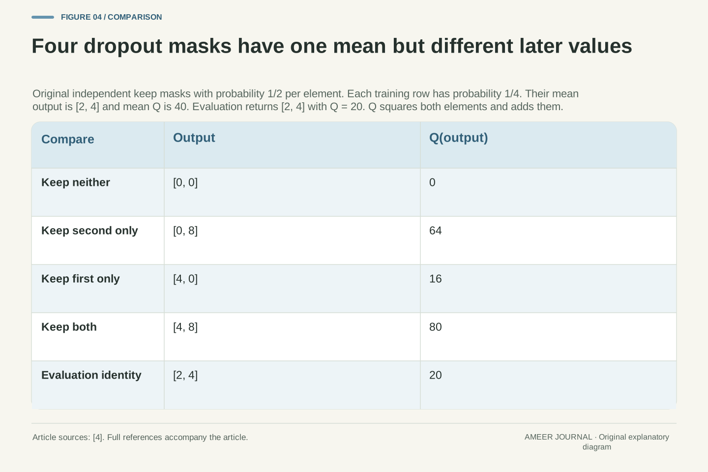
Take the input pair [2, 4]. For this example, each element is independently kept with probability one half. A kept element is doubled. There are four equally likely keep patterns: keep neither, keep only the second, keep only the first, or keep both. The corresponding outputs are [0, 0], [0, 8], [4, 0] and [4, 8]. No trainable weight needs to change for these outputs to differ.

In evaluation mode, the same dropout module returns [2, 4]. That pair is not one of our four training-mode outcomes. We have enumerated the possible masks mathematically; we have not sampled a random generator or measured a model. The example shows why a repeatable set of weights does not, by itself, specify the forward behavior.

For ordinary PyTorch Dropout, training applies random zeroing with probability p and scales retained elements by 1/(1−p); evaluation applies the identity map [4]. This distinction is controlled by module mode rather than by whether surrounding parameter tensors request gradients.

Specify input v=[2,4], p=1/2 and independent Bernoulli keep indicators m₁,m₂. The training output is [4m₁,8m₂]. Enumerating masks (0,0), (0,1), (1,0) and (1,1) yields [0,0], [0,8], [4,0] and [4,8], each with probability 1/4. Evaluation instead returns v exactly. No parameter update appears anywhere in this construction.

This is an analytic enumeration of a declared two-element example, not a reproducibility test of a seeded framework run. It establishes that fixed parameter values and fixed deterministic forward behavior are different properties. It does not imply that every model contains dropout, that every dropout variant uses this same element structure, or that one observed output difference can identify dropout as the sole cause.

Average the four dropout outputs one position at a time. The first position averages to 2 and the second to 4. That matches the evaluation output. The scaling rule preserves the expected value of each element in this example, but an average is not the same thing as every possible result.

To see why that matters, add a simple later calculation: square both elements and add them. Applied to the four training outputs, this gives 0, 64, 16 and 80. Their average is 40. Applied once to the evaluation output [2, 4], it gives 4+16=20. The later calculation produces different answers depending on whether we average before or after applying it.

This does not show that dropout is good or bad, or that a real model’s evaluation loss must be lower. Our square-and-add rule is an invented calculation. It shows the narrower mathematical limit: preserving an average at one location does not establish equal behavior after every later transformation. A model’s actual task results still need their own evaluation.

The four-mask distribution has E[ṽ]=[2,4], equal to the evaluation identity output. Now define the original downstream function Q(u)=u₁²+u₂². Across the four training outputs, Q takes values 0,64,16,80, so E[Q(ṽ)]=40. In contrast, Q(E[ṽ])=Q([2,4])=20.

This exact counterexample prevents an invalid inference from elementwise expectation preservation to equality after an arbitrary downstream transformation. Averaging and this nonlinear Q do not commute. The result follows from the stated finite distribution; it is not estimated from trials and does not depend on an unreported dataset.

Q is not presented as the loss of a real neural network. The example therefore supplies no universal ordering of training and evaluation losses, no accuracy prediction and no recommendation for a dropout probability. Its purpose is to separate a property of the dropout output’s expectation from a claim about the complete model. Evaluation mode selects a defined forward behavior; whether that behavior succeeds on the intended task is a further question.

A model can store more than weights. PyTorch distinguishes parameters from buffers, and its Module documentation gives a batch-normalization running mean as an example of a buffer [2]. Such a value can be part of the model’s saved state without being a weight that an optimizer learns through gradients.

BatchNorm1d illustrates the difference. With its usual tracking option enabled, it maintains running estimates of the mean and variance during training, then uses those estimates during evaluation [3]. It can also have learnable scale and offset parameters. Preventing gradients for the scale and offset does not, on its own, tell the module to stop maintaining the running estimates.

That distinction matters when someone says that the model did not change. They may have compared only parameter values. For a model containing this layer, selected buffers can still have changed. Conversely, a buffer change is not proof that a frozen parameter was updated. Inspect the kind of value and the rule that changes it before deciding which part of the training setup needs attention.

Module state is broader than the set of learnable parameters. PyTorch’s buffer registration documentation identifies BatchNorm running_mean as a non-parameter state value; persistent buffers are normally included alongside parameters in state_dict [2]. A gradient flag on parameters does not define all state transitions performed during a forward pass.

Use BatchNorm1d with affine=True and track_running_stats=True. The affine scale γ and offset β are learnable parameter vectors. The running mean and variance are tracked statistics, updated during training and used during evaluation [3]. Freezing γ and β does not change the module’s training flag or disable its documented running-statistic rule.

This example should not be generalized to every normalization layer or every transformer architecture. Nor do the two named buffers exhaust all possible module state. The point is a distinction of mechanisms: gradient-based parameter updates and forward-pass maintenance of buffers can occur under different controls. Comparing only the former cannot establish that the entire stored state is unchanged.

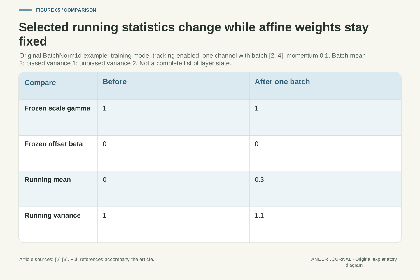
Set up one BatchNorm1d channel with tracking enabled. Freeze its scale at 1 and offset at 0. Start with running mean 0 and running variance 1, and choose momentum 0.1. Our training batch contains the two values 2 and 4. Their mean is 3.

The squared distances from that mean are 1 and 1. Dividing their sum by the batch size, 2, gives variance 1. Dividing instead by one less than the batch size gives variance 2. PyTorch documents the first, biased estimate for the training forward calculation and the second, unbiased estimate for the running-variance update [3]. Mixing these two denominators would give the wrong running result.

The new running mean is 0.9×0+0.1×3=0.3. The new running variance is 0.9×1+0.1×2=1.1. The frozen scale and offset remain 1 and 0. These selected stored statistics have changed even though the two named parameters have not. We are calculating statistics only, not reporting normalized outputs or running an actual layer.

Specify one channel, batch [2,4], affine=True, track_running_stats=True, frozen γ=1 and β=0, initial running mean 0, initial running variance 1 and fixed momentum m=0.1. The batch mean is 3 and the sum of squared centered deviations is 2.

The forward variance estimate divides by N=2, yielding 1. The unbiased estimate divides by N−1=1, yielding 2. PyTorch BatchNorm1d documents this distinction: training normalization uses the biased estimate, whereas the running-variance update uses the unbiased estimate [3]. The update convention is (1−m) times the old statistic plus m times the current statistic.

Therefore running_mean becomes 0.3 and running_var becomes 1.1, with γ and β unchanged. Momentum here is the BatchNorm averaging argument, not optimizer momentum; momentum=None would specify another averaging regime [3]. The example reports selected statistics rather than all layer state or epsilon-dependent normalized outputs. With track_running_stats=False, the documentation describes batch-statistic use during evaluation too, so that alternative configuration must not inherit this example’s evaluation assumptions.

The word evaluation can suggest that all learning machinery has stopped. In PyTorch, eval chooses a module’s evaluation behavior. The documentation explicitly separates it from no_grad [1, 2]. For dropout, that selects the identity behavior. For our tracked batch-normalization example, it selects use of the stored running statistics [3, 4].

Whether derivatives are recorded is still a separate question. If a calculation runs in ordinary grad mode with the needed trainable inputs, selecting evaluation behavior does not itself erase the gradient route. Likewise, selecting training behavior does not automatically unfreeze a weight whose gradient flag remains disabled.

This gives useful combinations rather than one universal switch. A pure scoring pass may need evaluation behavior and no gradient recording. Another calculation may deliberately need derivatives while retaining evaluation behavior. The correct combination follows from the task. If a program changes a mode temporarily, it should also restore the intended setup before the next operation; a successful-looking output does not show which controls were active.

Module.eval is equivalent to selecting training mode False, and the autograd documentation describes this as orthogonal to no-grad and inference modes [1]. Module mode affects only modules that implement mode-dependent behavior [2]. It does not globally disable differentiation or select an optimizer parameter set.

Consequently, eval plus ordinary grad mode can retain required derivative paths, while train plus no_grad can use training-specific forward behavior without recording those operations. In the latter case, no_grad alone does not convert Dropout to identity or freeze the tracked BatchNorm statistics described above [1–4]. Similarly, train does not reset frozen parameter flags to trainable.

A routine scoring pass and a calculation that needs input or parameter derivatives can legitimately use different combinations. The task must specify the desired module behavior and derivative scope independently. This article does not provide a universal wrapper for arbitrary custom modules; their behavior requires inspection. Mode labels are meaningful only alongside the actual module definitions, current flags and recording context.

Return to the batch-normalization example. If we feed a new batch through the layer with training behavior still selected, its tracked statistics can move toward that batch even if we never perform a weight update. That is why checking for optimizer steps alone is not enough to describe what a validation pass did.

PyTorch’s autograd guidance specifically mentions selecting evaluation mode to avoid updating batch-normalization running statistics on validation data [1]. In our tracked example, the intended evaluation pass uses the previously stored estimates. Disabling gradient recording can be a separate choice when we do not need derivatives.

The records should distinguish the state used to score the data from the state afterward. If the purpose is to compare two checkpoints, quietly modifying one during the comparison changes what is being compared. This is a question about the experiment’s definition, not proof that any particular result is invalid. It also does not replace selecting a suitable task metric or keeping evaluation data appropriate to the actual question [5].

A forward pass can mutate tracked statistics without any optimizer step. For the declared BatchNorm configuration, leaving training behavior active while processing validation data updates running buffers. A parameter-only comparison can therefore miss a state change that affects later evaluation.

PyTorch’s guidance explicitly identifies avoiding BatchNorm running-statistic updates on validation data as a reason to set evaluation mode [1]. The scoring protocol should state both the module-mode policy and whether autograd recording is required. These answer different questions; neither should be inferred solely from the absence of a backward call or optimizer step.

For a checkpoint comparison, define the input state and whether the evaluation procedure may change it. If selected state is intended to remain fixed, compare independent captured values before and after the pass. This is an experimental-design requirement for the stated comparison, not a claim that all evaluation protocols prohibit adaptation. Task quality remains separate: the Transformers guide describes explicitly computing a task metric rather than treating training-loop completion as the metric [5].

A project may first train a small final component, then decide to adjust an earlier component too. That change affects more than the name of a training phase. The newly trainable weight needs an update rule that includes it and a recorded path from the loss back to it.

Our two scalar arrangements make this concrete. When only b learns, the fixed feature 6 is sufficient. When a learns through fixed b, the multiplication by b must remain on a recorded derivative path. Reusing the first arrangement’s no-grad boundary in the second arrangement would remove something the new plan needs.

The same review should state which modules use training behavior and which stored statistics are allowed to change. There is no need to guess from a label such as feature extraction or fine-tuning. Write down the actual weight set, gradient settings, recording boundaries and module behavior. The change is then reviewable before judging task results, and any later comparison can say which setup produced each checkpoint.

A transition between training phases should define a new parameter-update set and re-evaluate required graph connectivity. In the scalar fixed-prefix case, b alone needs a gradient from a constant feature. In the fixed-suffix case, a needs the loss derivative to traverse multiplication by b. Reusing the same no-grad placement across those configurations is not semantically neutral.

The new plan also needs an explicit module-mode and buffer-update policy. A choice to train another parameter does not itself specify whether dropout is active or tracked statistics should adapt. Conversely, a change in module behavior does not add a tensor to the optimizer or establish its gradient eligibility.

This is a review framework rather than executable advice for every optimizer. Details such as existing optimizer state, previously accumulated gradients and custom mutations are outside the scalar fixture and must be handled by the actual implementation. Keeping those assumptions visible prevents the simplified teaching example from being mistaken for a complete phase-transition procedure.

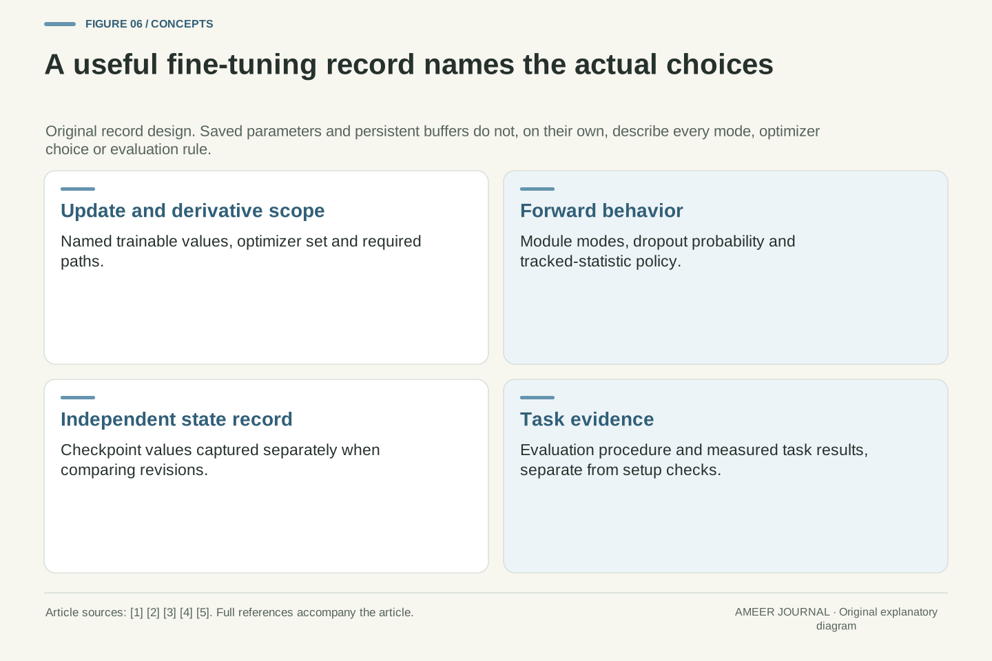
A useful record should say what was adapted, which weights could change, which derivative paths were needed and which modules used training behavior. For the batch-normalization example, it should also record the tracking option and averaging rule. For the dropout example, record its probability and the mode used for scoring.

Saved tensor values do not automatically describe all those choices. PyTorch’s state_dict includes parameters and persistent buffers, but its documentation says the returned dictionary contains references to the module’s values [2]. Keeping that dictionary in memory is therefore not, by itself, a frozen historical copy for a before-and-after comparison. Use an independent captured record when a comparison requires one.

Finally, keep the conclusion proportional to the evidence. Unchanged weights establish something about weights; a working gradient path establishes something about the requested calculation. Neither proves that the model is useful on its task. The small examples here make the controls visible so that later measurements can be interpreted with the right configuration in view.

Record the intended trainable parameter set, actual update set, gradient flags, required derivative paths, recording boundaries and module-mode policy. Include relevant configuration such as Dropout probability, BatchNorm affine/tracking settings, averaging argument and normalization epsilon when reproducing normalized outputs. Retain the checkpoint identity and evaluation procedure alongside task measurements.

Module.state_dict includes parameter values and persistent buffers, but its returned mapping is shallow and contains references [2]. An in-memory state_dict alone is not an immutable historical snapshot. Nor should it be treated as a complete record of training flags, optimizer configuration or the surrounding experiment. Comparisons requiring old values need an independent captured representation.

The article’s three fixtures establish narrower facts: a fixed suffix can carry a required gradient, training-mode dropout can vary without weight updates, and tracked normalization buffers can change while affine parameters remain fixed. None establishes task accuracy or runtime performance. Those conclusions require separate measurements made under a documented configuration, with the evidence attached to the actual model and evaluation data.